An up-to-date version of the package is available on https://github.com/ChHaeni/bLSmodelR.

Description

The package bLSmodelR provides functions to set up and run a backward Lagrangian stochastic (bLS) dispersion model with the statistical software R.

bLS Model

The model is a first-order Lagrangian stochastic model that is run in backward mode (i.e. backward in time) assuming horizontally homogeneous and vertically inhomogeneous Gaussian turbulence. The model is based on the paper published by Flesch et al. (2004). The basis of the model calculation is a generalized Langevin equation given as
du_i = a_i(x, u)*dt + b_ij(x, u)*dξ_j
dx_i = u_i*dt
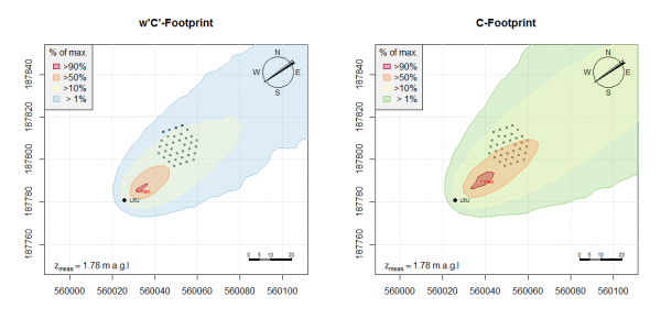
where dξ is a random increment from a Gaussian distribution N(0, dt). The indices i, j = 1, 2, 3 represent the alongwind (x), crosswind (y) and vertical axis (z) of the rotated coordinate system. x_i and u_i are position (x, y, z) and velocity (u, v, w) of the trajectory at time t. An ensemble of upwind trajectories is calculated starting from the sensor position x = (0, 0, z_meas-d) and the position and velocity of trajectory touchdowns on ground (i.e. on a horizontal plane at z = z₀ + d, where the modelled, average wind speed equals 0 m/s.) are recorded to calculate the sensor concentration to source strength relationship as the sum of the inverse touchdown velocities, summed over all touchdowns within the source
C/E = 2/N_traj*Σ_insideSource(1/w_TD)
where C represents the sensor concentration in mass per m³ and source areas are defined as homogenously emitting sources, having emission rate E in mass per m² and sec. As a consequence, the C/E relationship is expressed in s/m. Analogously, the flux to source strength ratios (<u'C'>/E, <v'C'>/E, <w'C'>/E) are calculated, mainly for completeness and for possible vertical flux footprint corrections. Trajectories touching ground are perfectly reflected and their velocities are reversed to maintain covariances past reflection. Therefore, no deposition is modelled when trajectory touchdown happens. Furthermore, this model is not capable of modelling chemistry, and trace gases have to be assumed to be inert within the relevant travelling time. For further details on the model and the concentration to emission rate relationship, see Flesch et al. (2004), Flesch (1996) and partly Flesch et al. (1995).

References

Flesch, T. K., J. D. Wilson, et al. (1995). “Backward-time Lagrangian stochastic dispersion models and their application to estimate gaseous emissions.” Journal of Applied Meteorology 34(6): 1320-1332.

Flesch, T. K. (1996). “The footprint for flux measurements, from backward Lagrangian stochastic models.” Boundary-Layer Meteorology 78(3-4): 399-404.

Flesch, T. K., J. D. Wilson, et al. (2004). “Deducing ground-to-air emissions from observed trace gas concentrations: A field trial.” Journal of Applied Meteorology 43(3): 487-502.

WindTrax Software. Available at http://www.thunderbeachscientific.com.